A practical introduction to Diff-Pruning for BERT

In this article I would like to give a short introduction for an elegant technique to make finetuning of large language models more storage efficient. From my own experience it is often the case that one has several instances of BERT stored on disk which only differ in terms of how much the weights were changed during task-adaptation. Diff-Pruning, which was developed by Guo et. al. in 2021 is a training technique which aims at tackling this problem. The basic idea of Diff-Pruning is to limit the amount of weights which are adapted during finetuning of a pre-trained model and to only store the difference of weights compared to their pre-trained state. The loss in performance compared to full finetuning was shown to be very minimal even with only .5% of the parameters of a full BERT_large model.

I came across Diff Pruning when I was looking at different sparsification techniques for a research project I am involved in. Unfortunately the code from the authors was set up in a way that it was difficult for me to integrate and expand which is why I decided to create my own Pytorch implementation from scratch. After a quick conceptual overview of the ideas presented in the paper, I will use my re-implementation in this article to explain how Diff-Pruning works in practice. The code from the original paper can be found on github.

What is Diff-Pruning

As already mentioned Diff-Pruning tries reduce the number of weights that get changed during finetuning of a pre-trained language model like BERT. It is important to note that it does not try to reduce or change the pre-trained model weights in any way. For this reason, a first important step for Diff-Pruning is to not think of just the set of model weights θ_pre that get changed during finetuning to task-specific θ_τ but to think of separate fixed pre-trained weight values θ_pre and task-specific “diff”-values δ_τ.

$$\theta_\tau = \theta_{pre} + \delta_\tau$$

instead of

$$\theta_{pre} \rightarrow \theta_\tau$$

The initial state of all weights in δ_τ is 0. We now want to limit the number of δ_τ,i which change to non-zero value during training. This constraint can be expressed as a L0 penalty in the loss function.

$$L(.) + \lambda \sum_{i=1}^{d} \mathbf{1}\big\{\delta_{\tau,i} \neq 0\big\}$$

For the set of parameters δ_τ the term 1{δ_τ,i≠0} equals 1 if δ_τ,i is non-zero. L is some Loss function, d represents the total number of parameters in the model and λ is a hyperparameter to control the degree of regularization. Since this penalty term is not differentiable however, it poses a challenge for training using gradient techniques. Thankfully there is a solution to this problem which was initially proposed by Louizos et. al. in 2018. They approximate the L0 objective via stochastic gates to make it differentiable. Stochastic gates in neural networks make use of the reparameterization trick (Kingma and Welling, 2014). Explaining the details about how it works would go beyond the scope of this article but there is a great many resources only which do just that, for example this one.

L0 Regularization

In principle, approximate L0 regularization works as follows:

1. Construct a mask z via a parametrized distribution called hard-concrete distribution

$$\begin{aligned} s &= \operatorname{Sigmoid}\big(\log u - \log(1 - u) + \log \alpha\big), \quad u \sim \mathcal{U}(0, 1) \\ \bar{s} &= s(r - l) + l \\ z &= \min(1, \max(0, \bar{s})) \end{aligned}$$

u is drawn from a uniform distribution and log(α) is the distribution parameter which is optimized together with the model weights during training. Typically for each parameter value in the model, a separate value for log(α) is learned. l and r are fixed hyperparameters which are typically set to -1.5 and 1.5 for Diff-Pruning. (Remark: the distribution features a second learnable parameter β which was disregarded, i.e. set to 1 for Diff-Pruning, I assume to simplify the calculations)

2. The z-mask which will be either 0 or 1 for the most part due to the hard sigmoid gate. It is incorporated in the model parameters as follows:

$$\theta_{new} = \theta \odot z$$

3. The L0 penalty term added to the loss is

$$\lambda \sum_{i=1}^{d} \operatorname{Sigmoid}\Big(\log \alpha_i - \log\Big(-\frac{l}{r}\Big)\Big)$$

4. At inference time we can remove the random part from z which was required for gradient-based training and make it deterministic by setting z to

$$\min(1, \max(0, \operatorname{Sigmoid}(\log \alpha)(r - l) + l))$$

For anyone who is interested how differentiable L0 regularization works in detail I recommend the paper from Louizos et. al. as well as the paper about the underlying distribution for categorical stochastic nodes by Maddison et. al. from 2017.

Below I included a simple visualization that shows how the PDF of the hard-concrete distribution changes for different values of alpha

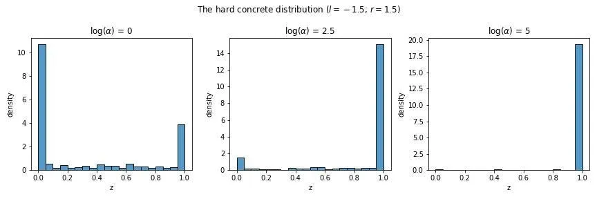
The smaller the parameter α the more likely z is to be equal to 0. This is why for Diff-Pruning α is typically initialized with a high value.

Diff-Pruning Training Procedure

By using this technique of differentiable L0 regularization we now have all the tools needed to implement the Diff-Pruning training procedure. We extend our loss function with the L0 penalty

$$L(.) + \lambda \sum_{i=1}^{d} \operatorname{Sigmoid}\Big(\log \alpha_i - \log\Big(-\frac{l}{r}\Big)\Big)$$

With the learned z mask the finetuned weights for diff pruning are now constructed as follows

$$\theta_\tau = \theta_{pre} + z_\tau \odot \delta_\tau$$

Implementing the weights in this way in Pytorch might seem a bit tricky at first, however since Pytorch 1.9 there is a very elegant way to do this with parametrizations. Parametrizations allow you to add operations to weights which are computed during each forward pass before the weights themselves are used to compute outputs for the next layer. For details I recommend the official tutorial which helped me a lot for the first implementation.

Just as with custom layers, weight parametrizations are defined by creating a new class which inherits from torch.nn.Module. My implementation for a particular δ_τ,i matrix looks as follows

class DiffWeight(nn.Module):
    """
    Implementation of diff pruning weights using pytorch parametrizations
    https://pytorch.org/tutorials/intermediate/parametrizations.html
    """
    def __init__(
        self,
        weight: torch.Tensor,
        alpha_init: Union[float, int],
        concrete_lower: Union[float, int],
        concrete_upper: Union[float, int]
    ):
        super().__init__()
        self.concrete_lower = concrete_lower
        self.concrete_upper = concrete_upper
        
        weight.requires_grad = False
        self.register_parameter("finetune", Parameter(torch.clone(weight)))
        self.register_parameter("alpha", Parameter(torch.zeros_like(weight) + alpha_init))
        
    def forward(self, X):
        diff = (self.finetune - X).detach()
        return (self.finetune - diff) + self.z * (self.finetune - X)
    
    @property
    def z(self) -> Parameter:
        return self.dist(self.alpha)

    def dist(self, x) -> torch.Tensor:
        return concrete_stretched(
            x,
            l=self.concrete_lower,
            r=self.concrete_upper,
            deterministic=(not self.training)
        )

In the forward method you define which operations are performed on the original weights X before they are used on the layer inputs. As the diff-weights are initially all 0 and 0s are usually a problem for gradient-based learning I did not implement

$$\theta_\tau = \theta_{pre} + z_\tau \odot \delta_\tau$$

directly but rather defined the weight parametrization as

$$\begin{aligned} \text{temp} &= (\theta_{full} - \theta_{pre}) \\ \theta_\tau &= \theta_{full} - \text{temp} + z_\tau * (\theta_{full} - \theta_{pre}) \end{aligned}$$

Here θ_full := θ_pre + δ_τ are the combination of pre-trained weight values and diff values and can be thought of as full finetuned weights. The gradient then gets calculated based on θ_full but since we store the original pre-trained weight values, we can recover δ_τ := (θ_full - θ_pre) in each step.

The Weight Class can now be very easily added to a certain parameter in the model with just one line of code (5 lines if you care about formatting)

parametrize.register_parametrization(
    module_name,
    param_name,
    DiffWeight(param, alpha_init, conc_upper, conc_lower)
)

If we do this for each parameter in the pre-trained language model we have our Diff-Pruning model!

What remains for Diff-Pruning to work is the calculation of the loss and more specifically the calculation of the L0 penalty term. Below is an example how this can be implemented.

sparsity_pen = 1.25e-7

loss = loss_fn(outputs, labels.to(self.device))

l0_pen = 0.
for module_name, base_module in get_encoder_base_modules(return_names=True):
    for par_list in list(base_module.parametrizations.values()):
        l0_norm = get_l0_norm_term(par_list[0].alpha, log_ratio)
        l0_pen += (l0_norm * sparsity_pen)
loss += l0_pen

During each step we calculate our normal task loss with with some loss function loss_fn. We then collect our L0 penalty terms from each weight by looping over all modules that contain parameters directly (i.e. modules can be stacked hierarchically in pytorch so some of them might not contain any parameters directly but just other modules). get_encoder_base_modules is a method to retrieve those modules. Furthermore parameterizations in Pytorch are stored in a list as one weight can contain several of them which is why we need index [0] for object par_list.

Finally, get_l0_norm_term calculates the penalty term mentioned above.

def get_log_ratio(concrete_lower: float, concrete_upper: float) -> int:
    return 0 if (concrete_lower == 0) else math.log(-concrete_lower / concrete_upper)

def get_l0_norm_term(alpha: torch.Tensor, log_ratio: float) -> torch.Tensor:
    return torch.sigmoid(alpha - log_ratio).sum()

From the combined loss we can then do the backward pass to update all our weights as well as the alpha values.

Magnitude Pruning

In principle with these building blocks Diff-Pruning can be integrated into a typically Pytorch model pipeline. However there is one step left in Diff-Pruning which I haven’t mentioned so far. With the training procedure outlined above it is not really possible to control the exact degree of sparsity in the δ values. This is why Guo et. al. apply magnitude pruning to the diff values after training for some epochs. In magnitude pruning you define an exact sparsity percentage, lets say 5%, and then keep only the top 5% of weights in terms of their magnitude.

For Diff-Pruning if you want the parameter count down to 5% or even lower, it is quite a big reduction from the first stage where the z-masks are trained (this resulted in around 20%-30% of parameters being zeroed out in my experiments). This is why it is important to keep training the model after the magnitude pruning step for some epochs. For this to work in my implementation I needed to create a new parameterization for this training procedure after magnitude pruning as now the z-masks are fixed and we just need to prune the remaining δ values.

class DiffWeightFixmask(nn.Module):
    
    def __init__(self, pre_trained: torch.Tensor, mask: torch.Tensor):
        super().__init__()
        self.register_parameter("pre_trained", Parameter(pre_trained, requires_grad=False))
        self.register_parameter("mask", Parameter(mask, requires_grad=False))
    
    def forward(self, X):
        return self.pre_trained + self.mask * X   

X here now represents a δ value for which gradient computation is active. All other parameters have requires_grad set to False. In the Mangitude Pruning step we now switch from our old parameterizations DiffWeight from above to this new parametrization by calculating the magnitude of our δ values and generating a mask which has zeroes everywhere where the magnitude is below our threshold. The code for this step looks as follows

def _get_cutoff(values, pct):
    k = int(len(values) * pct)
    return torch.topk(torch.abs(values), k, largest=True, sorted=True)[0][-1]            

diff_weights = torch.tensor([])
for base_module in get_encoder_base_modules():
    for n, par_list in list(base_module.parametrizations.items()):
        par_list[0].set_mode(train=False)
        diff_weight = (getattr(base_module, n) - par_list.original).detach().cpu()
        diff_weights = torch.cat([diff_weights, diff_weight.flatten()])
cutoff = _get_cutoff(diff_weights, pct)
for base_module in get_encoder_base_modules():
    for n, par_list in list(base_module.parametrizations.items()):
        pre_trained_weight = torch.clone(par_list.original)
        parametrize.remove_parametrizations(base_module, n)
        p = base_module._parameters[n].detach()
        diff_weight = (p - pre_trained_weight)
        diff_mask = (torch.abs(diff_weight) >= cutoff)
        base_module._parameters[n] = Parameter(diff_weight * diff_mask)
        parametrize.register_parametrization(
            base_module,
            n,
            DiffWeightFixmask(pre_trained_weight, diff_mask)
        )

We need to first loop over the parametrizations to get the δ values (i.e. diff weights) and store them in a list to calculate a cutoff value. We then do a second loop over the parameters where we remove our existing parametrizations and register the new parametrizations with a fixed mask.

We then continue training the model for some epochs. Below you can find an example how Diff-Pruning and Magnitude Pruning work together for a simple parameter matrix.

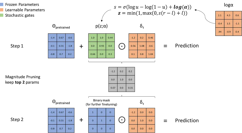
There is also an extension to Diff-Pruning where an additional scalar z-values is learned per parameter matrix to encourage entire parameter blocks to be zeroed out. Since it works just the same as before I would not go into detail here and refer interested readers to the paper by Guo et. al.

Final thoughts

You can find my code on github and some experiments I did on tensorboard (TensorBoard.dev has since shut down). The code is a bit more extensive than what is shown in the article as I also implemented structured Diff-Pruning for example but I am happy to answer questions about it in the comment section. The tensorboard includes runs for two datasets GLUE-SST2 and a custom dataset where a job category needs to be predicted based on short biographies. Furthermore, I tested three different model versions:

• diff_pruning_fixmask: the regular (+structured) Diff-Pruning training procuedure I outlined in this article
• finetuning_fixmask: regular finetuning but with magnitude pruning after some epochs. This experiment shows that diff_pruning is important as with magnitude pruning only here we do not recover much of the accuracy.
• finteuning_no_fixmask: this is just regular finetuning as a reference baseline.

I hope with this article I was able to give you some insights into how Diff-Pruning works and how it can be implemented in Pytorch. Even though there have been new techniques with even better performance like FISH Mask (Sung et. al., 2021) I think Diff-Pruning has some potential for further research as an elegant way to sparsify large models.

References

[1] Guo, D., Rush, A., & Kim, Y. (2021). Parameter-efficient transfer learning with diff pruning. Annual Meeting of the Association for Computational Linguistics / International Joint Conference on Natural Language Processing, 4884–4896.

[2] Louizos, C., Welling, M., & Kingma, D. P. (2018). Learning sparse neural networks through l0 regularization. International Conference on Learning Representations.

[3] Kingma, D. P., & Welling, M. (2014). Auto-encoding variational bayes. International Conference on Learning Representations.

[4] Maddison, C. J., Mnih, A., & Teh, Y. W. (2017). The concrete distribution: A continuous relaxation of discrete random variables. International Conference on Learning Representations.

[5] Sung, Y.-L., Nair, V., & Raffel, C. (2021). Training neural networks with fixed sparse masks. ArXiv, abs/2111.09839.